Set the analysis domain
Define the horizontal grid extent from polygons representing the target area.
This page summarizes the Global Water-Cycle Model: core specifications, input data, three-dimensional model structure, hydrogeologic framework, transient analysis including evapotranspiration and snowmelt, and discharge validation.
The Global Water-Cycle Model is a wide-area water-cycle model for evaluating surface-water and groundwater flow at the global scale. It is built on GETFLOWS, the GEneral purpose Terrestrial fluid-FLOW Simulator. The model integrates globally available terrain, drainage, geology, soils, land use, vegetation, meteorology, and observations on a grid basis, and represents surface-water flow, groundwater flow, recharge, spring discharge, and evapotranspiration within a single three-dimensional model domain.
Defines ground-surface geometry and catchment conditions.
Sets surface-water boundaries and water-body conditions.
Assigns hydraulic properties from topsoil, cover layers, bedrock, weathering, and loosened zones.
Provides precipitation, potential evapotranspiration, and daily meteorological forcing.
The representative configuration shown here couples surface water and groundwater in GETFLOWS and uses a two-phase water-air formulation. Under average forcing conditions, the model evaluates a natural equilibrium state without anthropogenic water use.
| Name | Global Water-Cycle Model |
|---|---|
| Simulator | GETFLOWS, the GEneral purpose Terrestrial fluid-FLOW Simulator |
| Fluid system | Coupled surface-subsurface flow with two-phase water-air flow |
| Domain | Global land area from approximately 60°S to 84°N |
| Horizontal resolution | 10 arc-minutes × 10 arc-minutes, approximately 18.6 km × 18.6 km near the equator |
| Vertical discretization | 15 layers |
| Lower boundary | Elevation -3000 m |
| Analysis condition | Natural equilibrium under average forcing conditions, without anthropogenic water use |
| Steady meteorological forcing | Year-round constant forcing from CHELSA V2.1 precipitation and CHELSA V2.1 potential evapotranspiration corrected by an empirical coefficient of 0.65 |
| Fluid properties: water | Density 1,000 kg/m³, viscosity 1.0×10⁻³ Pa·s, compressibility 4.5×10⁻¹⁰ 1/Pa |
| Fluid properties: air | Density 1.22 kg/m³, viscosity 1.82×10⁻⁵ Pa·s, with compressibility inversely proportional to pressure |
| Boundary conditions | Standard atmospheric pressure at the atmosphere boundary, no-flow bottom and side boundaries, and tide fixed at MSL 0 m |
The model converts globally available external datasets, together with model-derived estimates and derivative datasets, into grid-level terrain, water-body, geology, soil, land-use, vegetation, meteorological, and observation information. This section focuses on the role of each dataset as model input.
The external data-source list is provided on a separate page.
| Category | Dataset | Role in the model |
|---|---|---|
| Meteorology and climate | Climate classification | Köppen-Geiger global climate classification is used to organize surface conditions and regional characteristics according to terrain and climate. |
| Meteorology and climate | Normal meteorology | CHELSA v2.1 precipitation and potential evapotranspiration are converted to annual mean daily values and used as steady forcing. |
| Meteorology and climate | Daily meteorology | ERA5 daily precipitation, air temperature, wind speed, surface pressure, relative humidity, and shortwave and longwave radiation are used as transient forcing. |
| Meteorology and climate | Future climate input | ISIMIP / CMIP6 GCM inputs are assigned to the global model for comparing future conditions. |
| Terrain and water system | Land elevation | AW3D30 is used as source information for the ground surface, terrain relief, and weathering-surface generation. |
| Terrain and water system | Bathymetry and ocean area | GEBCO is used to define marine cells, bathymetry, and boundary conditions including coastal areas. |
| Terrain and water system | River network and bed elevation | HydroSHEDS v1 accumulation area and elevation are used to organize river locations, river-bed elevations, and hydrologic terrain information. |
| Terrain and water system | Lake topography | HydroLAKES and GLOBathy are used to organize lake extent, lake-surface elevation, and lake-bed elevation. |
| Geology and soils | Topsoil and cover layers | SoilGrids sand, silt, clay content, and bulk density are used to classify topsoil and cover layers into hydraulic-property classes. |
| Geology and soils | Weathering and geomorphic surfaces | AW3D30-derived terrain, climate classification, hydraulic type, and weathering surfaces are combined to build the shallow-to-deep subsurface structure. |
| Geology and soils | Bedrock | USGS World Geologic Maps are reclassified into model geologic codes and used for deep hydraulic properties. |
| Geology and soils | Hydraulic properties | Hydraulic-property lists based on general and literature values connect geology, soils, and weathered zones to hydraulic-property classes. |
| Land use and vegetation | Land use | GLCLUC2019 is used to classify forest, cropland, built-up areas, water bodies, and other surface conditions. |
| Land use and vegetation | Vegetation type | ESA CCI PFT is used to classify forest types and provide vegetation conditions for forest evapotranspiration analysis. |
| Land use and vegetation | Canopy height | ETH Global Canopy Height 2020 is used when setting evapotranspiration and vegetation parameters in forest areas. |
| Land use and vegetation | Tree density | Crowther global tree-density data is combined with canopy height to represent forest structure in transient analysis. |
| Land use and vegetation | Leaf seasonality | GSI is calculated from ERA5 daily meteorology and used to represent leaf-on and leaf-off dates in forest and vegetation areas. |
| Land use and vegetation | Crop coefficients | ISIMIP3 crop calendars and ERA5 meteorological conditions are used to build crop coefficients and soil evaporation coefficients for FAO-56 and evapotranspiration conditions over cropland. |
| Observations | Observed river discharge | River-discharge time series such as GRDC-Caravan are compared with simulated discharge for model-performance diagnosis. |
This section covers the analysis domain, horizontal grid, surface conditions, and vertical layering.
Define the horizontal grid extent from polygons representing the target area.
Divide the target area at the specified horizontal resolution to create the computational grid.
Organize elevation, rivers, lakes, ocean areas, land use, meteorology, and vegetation on a grid basis.
Divide the domain vertically from the ground surface to the lower analysis boundary.
Classification information from geologic and soil maps is converted into hydraulic properties used in the simulation. The model organizes topsoil, water-body sediment, cover layers, weathered and loosened zones, and bedrock, then reflects these elements in hydraulic conductivity, storage, and unsaturated-zone water-retention properties.
| Item | Description | Representation in the model |
|---|---|---|
| Hydraulic conductivity | A value describing how easily water passes through geologic layers or soils. | Affects groundwater flow, river discharge, and recharge. |
| Anisotropy kv/kh | Difference between vertical and horizontal permeability. | Controls whether groundwater tends to flow laterally or infiltrate downward. |
| Effective porosity | Fraction of pore space participating in water movement. | Controls groundwater storage and flow velocity. |
| Two-phase flow properties | Water-retention properties when water and air occupy the same pore space. | Used to represent infiltration, evaporation, and retention in the unsaturated zone. |
| Specific storage | Water released or stored per unit pressure change. | Relevant to groundwater-level change and storage change. |
Topsoil, water-body sediment, cover layers, weathered and loosened zones, and bedrock have distinct hydraulic properties. The following tables summarize how each dataset is treated as a geologic or soil element and how it is reflected in model properties.
| Element | Content | Model property |
|---|---|---|
| Topsoil | Sand, silt and clay content, bulk density, and soil-water retention properties. | Sets near-surface infiltration, water retention, effective porosity, and storage. |
| Cover layers | Target areas are selected by geomorphic classification and overlaid with sand, silt and clay content and bulk density. | Assigns materials for shallow ground in plains, terraces, hills, and related settings separately from topsoil. |
| Water-body sediment | Classification of rivers, lakes, and ocean areas. | Represents locations where water exchanges between water bodies and the subsurface through infiltration and discharge. |
| Element | Content | Model property |
|---|---|---|
| Classification-surface rasters | Multiple base surfaces from shallow to deep zones are prepared from terrain elevation, summit-level surfaces, valley-bottom surfaces, and related inputs. | Overlaid with bedrock distribution to determine the degree of weathering and loosening with depth. |
| Depth-dependent properties | The same bedrock type is configured to be relatively more permeable near the surface and less permeable at depth. | Adds vertical hydraulic-property variation to horizontally distributed geologic classes. |
| 3D integration | Bedrock plan-view distribution is combined with weathering and loosening classification surfaces. | Creates a 3D hydrogeologic structure combining geologic classes and depth-dependent property changes. |
| Element | Content | Model property |
|---|---|---|
| Bedrock distribution | Bedrock read from geologic maps and supplemental distribution rules for ocean areas or insufficiently classified locations are organized under consistent rules. | Represents continuous deep geology across the full analysis domain. |
| Sedimentary rocks | Age and lithology of sedimentary rocks are organized. | Differences among sandstone, mudstone, carbonate rocks, and related lithologies are reflected in deep permeability and storage. |
| Volcanic rocks | Mafic, intermediate, felsic, and other lithologies and ages are organized. | Represents differences in groundwater flow and storage in volcanic-rock regions. |
| Plutonic and metamorphic rocks | Granitoids, gneisses, and other deep-basement rocks are organized. | Provides the deep structural background for regional groundwater flow. |
In the steady analysis, CHELSA V2.1 potential evapotranspiration is applied as year-round constant forcing. For discharge validation and seasonal diagnostics, the model uses daily meteorological data in transient analysis and sets evapotranspiration conditions for forest, cropland, and other land-use classes. In snowy regions, snow accumulation and snowmelt are treated separately, and model water input is given as rainfall plus snowmelt.
| Target | Main inputs and settings | Use in the model |
|---|---|---|
| Steady analysis | CHELSA v2.1 potential evapotranspiration × 0.65 | Corrected CHELSA-derived potential evapotranspiration is used as year-round constant forcing for the natural equilibrium state. |
| Transient forest analysis | ESA CCI PFT, canopy height, tree density, GSI-derived leaf-on and leaf-off dates, and daily meteorology | The forest-floor evaporation model and the canopy interception / transpiration model are combined to separately evaluate canopy interception, transpiration, and forest-floor evaporation. |
| Transient cropland and other analysis | Crop coefficients and soil evaporation coefficients for FAO-56, ISIMIP3 crop calendar, and ERA5 meteorological conditions | Reference evapotranspiration is calculated with FAO-56 Penman-Monteith, and transpiration and evaporation components over cropland and other surfaces are evaluated. |
| Transient snow and snowmelt analysis | Daily meteorology, rainfall, and snowmelt | In snowy regions, snow accumulation and snowmelt are included following the approach of Fukazawa and Tada (2024), and water input is organized as rainfall plus snowmelt. |
| Conversion to actual evapotranspiration | Evapotranspiration efficiency based on topsoil properties | Potential evapotranspiration is reduced according to topsoil properties and water conditions. Forest areas use the Feddes et al. (1978) root water-uptake model, while non-forest areas use evaporation efficiency based on Lehmann et al. (2018). |
| Application to the model | Water input, potential evapotranspiration, and actual evapotranspiration | Rainfall, snowmelt, interception, and evapotranspiration efficiency are applied as water exchanges in the coupled surface-water and groundwater simulation. |
For regions where observed discharge data such as GRDC-Caravan are available, the global model compares daily observed and simulated discharge in a consistent format. This section shows representative discharge time-series comparisons from different basins to evaluate reproducibility as a wide-area model.
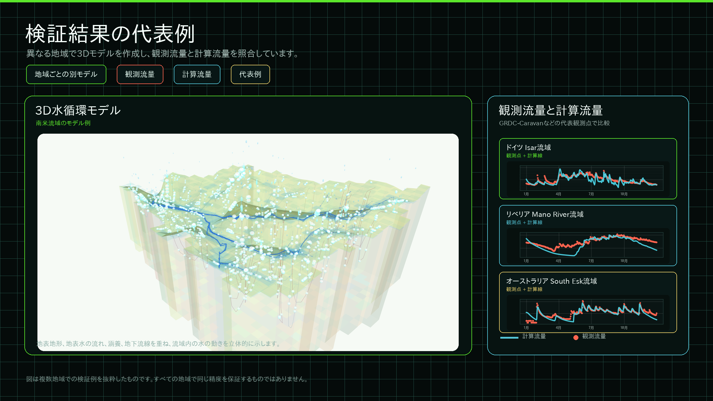
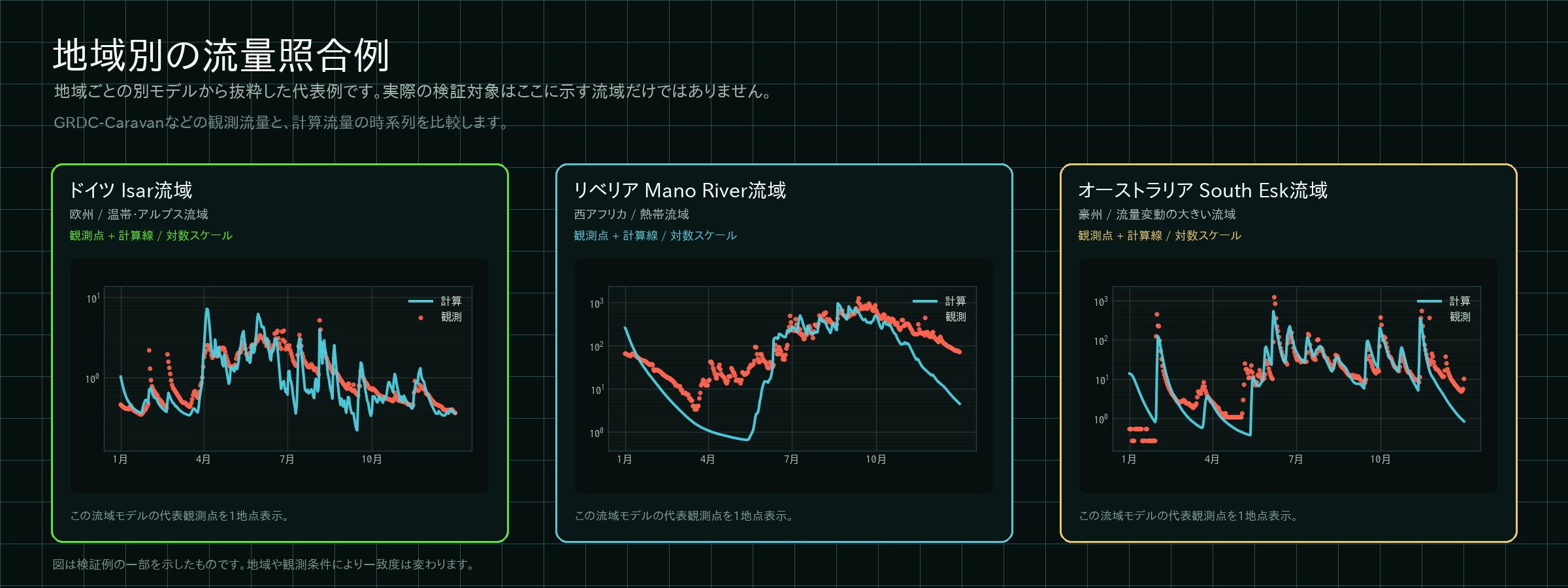
The figures show representative examples where observed and simulated discharge were compared using the same workflow across multiple regions. Site-specific reproducibility depends on available discharge data, basin area, river-channel representation, and the presence of dry or intermittent flow.
Model outputs can be organized as map layers and regional diagnostic reports. By overlaying input data and model results, the effects of terrain, geology, land use, and meteorological conditions on water-cycle quantities can be evaluated.
Evaluates groundwater-surface elevation relative to the ground surface and its spatial distribution.
G.L. mEvaluates spatial distribution of surface-water depth in rivers, lakes, and lowlands.
mEvaluates the degree to which the topsoil layer is filled with water.
-Quantifies water moving through rivers and over the land surface.
m³/dayEvaluates the direction and magnitude of water movement underground.
m³/dayEvaluates water supplied to groundwater from rainfall and related processes.
mm/dayShows the distribution and amount of water returning from the subsurface to the surface and rivers.
mm/dayEvaluates water returning to the atmosphere from the ground surface and water surfaces.
mm/dayEvaluates water returning to the atmosphere through the subsurface and unsaturated zone.
mm/dayOrganizes the ratio of actual evaporation to potential evaporation.
-Organizes precipitation contributing to runoff and recharge as a water-cycle quantity.
mmVisualizes the flow direction and flow conditions of surface water and groundwater.
flow linesWebmap lets users inspect terrain, land use, meteorological conditions, and computed water-cycle quantities incorporated in the Global Water-Cycle Model. The Webmap top page provides links to the public viewers and technical overview pages for each model.